plots.drag module

Plot the drag coefficiente as function of reynolds number of a sphere.

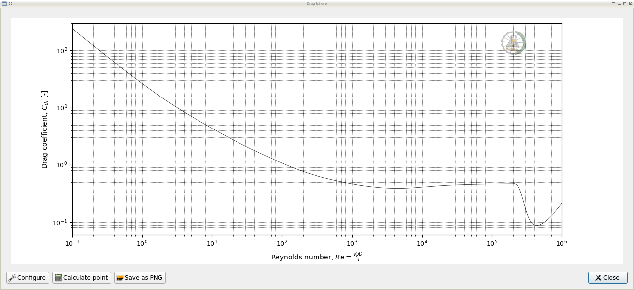
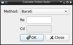
The diagram include all Reynolds number range, support for click interaction, let user save the chart as image and a dialog to calculate a individual point:

Configuration

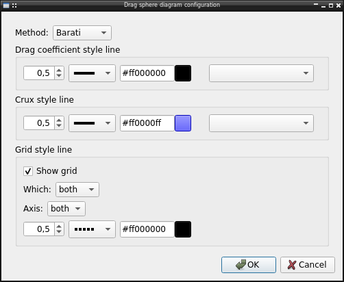
The diagram let user configure several options like:

• Equation to use, by default the Barati correlation, but it’s possible use one of available in lib.drag

• Line style used in plot

• Line style used in crux when use mouse

• Grid line visibility and style

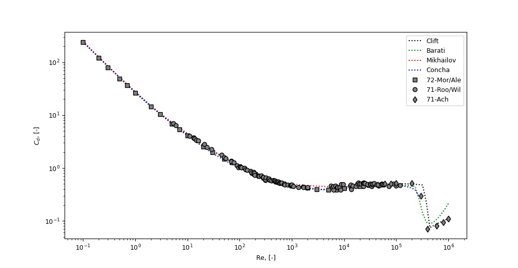
Example

Comparing some correlations with experimental data

from matplotlib import pyplot
from numpy import logspace

from lib.drag import Clift, Mikhailov, Concha, Barati

corr = {
    Clift: {"c": "black", "ls": ":"},
    Barati: {"c": "green", "ls": ":"},
    Mikhailov: {"c": "red", "ls": ":"},
    Concha: {"c": "blue", "ls": ":"}}

Re = logspace(-1, 6, 100)
for f, kw in corr.items():
    Cd = []
    for re in Re:
        try:
            v = f(re)
        except NotImplementedError:
            v = None
        Cd.append(v)
    pyplot.plot(Re, Cd, label=f.__name__, **kw)


# Experimental date
# Morsi, S.A., Alexander, A.J.
# An Investigation of Particle Trajectories in Two-Phase Flow Systems
# J. Fluid Mechanics 55(2) (1972) 193-208
# doi: 10.1017/S0022112072001806
Re = [0.1, 0.2, 0.3, 0.5, 0.7, 1, 2, 3, 5, 7, 10, 20, 30, 50, 70, 100, 200,
      300, 500, 700, 1000, 2000, 3000, 5000, 7000, 10000, 20000, 30000,
      50000]
Cd = [240, 120, 80, 49, 36.5, 26.5, 14.4, 10.4, 6.9, 5.4, 4.1, 2.55, 2, 1.5,
      1.27, 1.07, 0.77, 0.65, 0.55, 0.5, 0.46, 0.42, 0.4, 0.385, 0.39, 0.41,
      0.452, 0.4697, 0.488]
pyplot.plot(Re, Cd, ls='', marker="s", mec="k", mfc="grey", label="72-Mor/Ale")


# Roos, F.W., Willmarth, W.W.
# Some Experimental Results on Sphere and Disk Drag
# Amer. Inst. Aeronautics and Astronautics 9(2) (1971) 285-291
# doi: 10.2514/3.6164
Re = [5.33, 5.99, 11.0, 13.1, 13.2, 13.9, 14.6, 16.2, 21.1, 23.4, 29.1, 45.0,
      50.6, 54.4, 68.9, 68.9, 78.2, 88.1, 93.8, 101, 104, 108, 109, 124, 130,
      138, 163, 168, 170, 186, 186, 189, 190, 191, 193, 229, 229, 240, 258,
      280, 284, 286, 311, 312, 318, 358, 361, 364, 379, 409, 444, 468, 472,
      480, 500, 522, 532, 532, 557, 579, 588, 603, 644, 713, 727, 833, 932,
      984, 985, 985, 1000, 1000, 1070, 1330, 1650, 1690, 1950, 2000, 5570,
      5990, 6210, 6250, 6900, 7280, 7520, 8230, 8580, 8700, 9620, 13300, 13400,
      13900, 14700, 16800, 18000, 18700, 19500, 21200, 23100, 23600, 23700,
      24100, 24200, 25000, 28000, 31900, 32400, 33800, 35400, 35500, 38200,
      41800, 45900, 46800, 52400, 53500, 57500, 57700, 71900, 89000, 100000,
      118300]
Cd = [7.06, 6.41, 4.01, 3.76, 3.66, 3.59, 3.41, 3.29, 2.82, 2.48, 2.28, 1.79,
      1.58, 1.52, 1.35, 1.33, 1.27, 1.12, 1.03, 1.08, 1.05, 1.02, 1.03, 0.994,
      0.927, 0.907, 0.879, 0.799, 0.819, 0.799, 0.841, 0.778, 0.751, 0.799,
      0.732, 0.711, 0.710, 0.700, 0.721, 0.674, 0.646, 0.675, 0.592, 0.607,
      0.656, 0.627, 0.600, 0.632, 0.595, 0.579, 0.585, 0.578, 0.566, 0.572,
      0.547, 0.544, 0.543, 0.556, 0.552, 0.523, 0.520, 0.531, 0.525, 0.505,
      0.480, 0.485, 0.472, 0.466, 0.477, 0.485, 0.472, 0.483, 0.452, 0.436,
      0.440, 0.435, 0.427, 0.430, 0.460, 0.430, 0.390, 0.451, 0.460, 0.430,
      0.435, 0.429, 0.390, 0.490, 0.490, 0.460, 0.480, 0.400, 0.460, 0.452,
      0.510, 0.523, 0.500, 0.509, 0.511, 0.529, 0.455, 0.524, 0.520, 0.519,
      0.495, 0.500, 0.479, 0.457, 0.482, 0.504, 0.513, 0.485, 0.467, 0.468,
      0.503, 0.497, 0.480, 0.492, 0.451, 0.502, 0.467, 0.476]
pyplot.plot(Re, Cd, ls='', marker="o", mec="k", mfc="grey", label="71-Roo/Wil")


# Achenbach, E.
# Experiments on the Flow Past Spheres at Very High Reynolds Numbers
# J. Fluid Mech. 54(3) (1972) 565-575
# doi: 10.1017/S0022112072000874
# Selected point of figure 4, the paper don't report the experimental data
Re = [4.4e4, 6e4, 8e4, 1e5, 2e5, 3e5, 4e5, 6e5, 8e5, 1e6]
Cd = [0.48, 0.5, 0.51, 0.52, 0.52, 0.3, 0.07, 0.08, 0.095, 0.11]
pyplot.plot(Re, Cd, ls='', marker="d", mec="k", mfc="grey", label="71-Ach")


pyplot.ylabel("$C_d$, [-]")
pyplot.xlabel("Re, [-]")
pyplot.xscale("log")
pyplot.yscale("log")
pyplot.legend()
pyplot.show()

API Reference

The module include all related moody chart functionality

• Drag: Chart dialog

• CalculateDialog: Dialog to calculate a specified point and its configuration

• Config: Drag sphere chart configuration

plots.drag.translate(context: str, sourceText: str, disambiguation: str = None, n: int = -1) → str

class plots.drag.Config(config=None, parent=None)

Bases: QWidget

Drag sphere chart configuration

Methods

value(config)

Update ConfigParser instance with the config

TITLE = 'Drag Sphere chart'

TITLECONFIG = 'Drag sphere diagram configuration'

__init__(config=None, parent=None)

value(config)

Update ConfigParser instance with the config

class plots.drag.Drag(parent=None)

Bases: Chart

Drag sphere chart dialog

Attributes:

note

Methods

calculate()	Define the functionality when click the calculate point button
clearCrux()	Remove crux and note if exist
click(event)	Update input and graph annotate when mouse click over chart
config()	Initialization action in plot don't neccesary to update in plot
createCrux(Re, Cd)	Create a crux in selected point of plot and show data at bottom right corner
plot()	Plot the drag chart using the indicate method
widgetConfig

title = 'Drag Sphere'

widgetConfig

alias of Config

locLogo = (0.8, 0.85, 0.1, 0.1)

note = None

config()

Initialization action in plot don’t neccesary to update in plot

click(event)

Update input and graph annotate when mouse click over chart

static _txt(Re, Cd)

clearCrux()

Remove crux and note if exist

createCrux(Re, Cd)

Create a crux in selected point of plot and show data at bottom right corner

plot()

Plot the drag chart using the indicate method

calculate()

Define the functionality when click the calculate point button

class plots.drag.CalculateDialog(parent=None)

Bases: QDialog

Dialog to calculate a specified point

Methods

calculate()

Calculate point procedure

__init__(parent=None)

calculate()

Calculate point procedure