lib.drag module

Module for drag coefficient correlations, for now only implemented the sphere drag correlation

dragSphere(): Function to implement the drag coeficient for smooth spheres including all available methods:

• Barati()

• Clift()

• Ceylan()

• Almedeij()

• Morrison()

• Morsi()

• Khan()

• Flemmer()

• Haider()

• Turton()

• Concha()

• Swamee()

• Cheng()

• Terfous()

• Mikhailov()

Plot the drag coefficiente as function of reynolds number of a sphere.

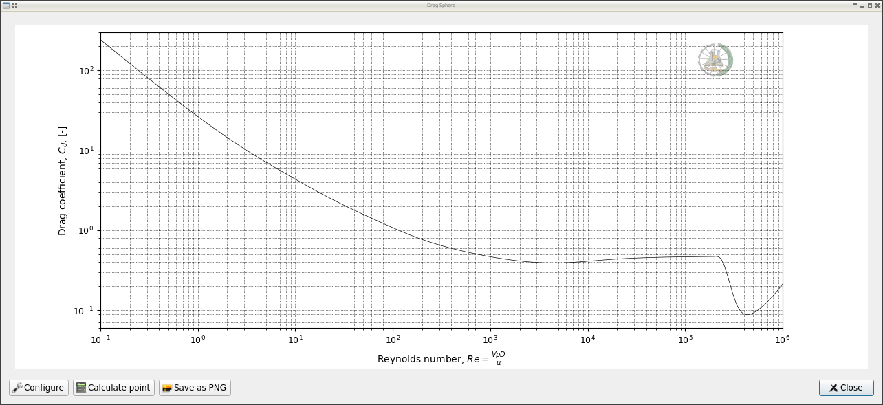
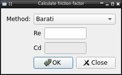
The diagram include all Reynolds number range, support for click interaction, let user save the chart as image and a dialog to calculate a individual point:

Configuration

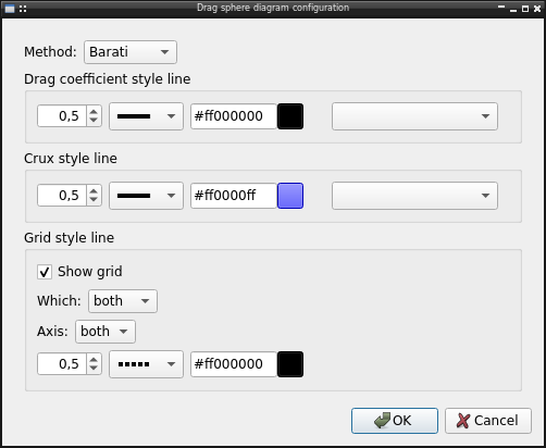
The diagram let user configure several options like:

• Equation to use, by default the Barati correlation, but it’s possible use one of available in lib.drag

• Line style used in plot

• Line style used in crux when use mouse

• Grid line visibility and style

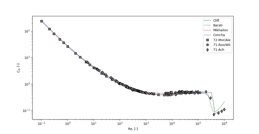
Example

Comparing some correlations with experimental data

from matplotlib import pyplot
from numpy import logspace

from lib.drag import Clift, Mikhailov, Concha, Barati

corr = {
    Clift: {"c": "black", "ls": ":"},
    Barati: {"c": "green", "ls": ":"},
    Mikhailov: {"c": "red", "ls": ":"},
    Concha: {"c": "blue", "ls": ":"}}

Re = logspace(-1, 6, 100)
for f, kw in corr.items():
    Cd = []
    for re in Re:
        try:
            v = f(re)
        except NotImplementedError:
            v = None
        Cd.append(v)
    pyplot.plot(Re, Cd, label=f.__name__, **kw)


# Experimental date
# Morsi, S.A., Alexander, A.J.
# An Investigation of Particle Trajectories in Two-Phase Flow Systems
# J. Fluid Mechanics 55(2) (1972) 193-208
# doi: 10.1017/S0022112072001806
Re = [0.1, 0.2, 0.3, 0.5, 0.7, 1, 2, 3, 5, 7, 10, 20, 30, 50, 70, 100, 200,
      300, 500, 700, 1000, 2000, 3000, 5000, 7000, 10000, 20000, 30000,
      50000]
Cd = [240, 120, 80, 49, 36.5, 26.5, 14.4, 10.4, 6.9, 5.4, 4.1, 2.55, 2, 1.5,
      1.27, 1.07, 0.77, 0.65, 0.55, 0.5, 0.46, 0.42, 0.4, 0.385, 0.39, 0.41,
      0.452, 0.4697, 0.488]
pyplot.plot(Re, Cd, ls='', marker="s", mec="k", mfc="grey", label="72-Mor/Ale")


# Roos, F.W., Willmarth, W.W.
# Some Experimental Results on Sphere and Disk Drag
# Amer. Inst. Aeronautics and Astronautics 9(2) (1971) 285-291
# doi: 10.2514/3.6164
Re = [5.33, 5.99, 11.0, 13.1, 13.2, 13.9, 14.6, 16.2, 21.1, 23.4, 29.1, 45.0,
      50.6, 54.4, 68.9, 68.9, 78.2, 88.1, 93.8, 101, 104, 108, 109, 124, 130,
      138, 163, 168, 170, 186, 186, 189, 190, 191, 193, 229, 229, 240, 258,
      280, 284, 286, 311, 312, 318, 358, 361, 364, 379, 409, 444, 468, 472,
      480, 500, 522, 532, 532, 557, 579, 588, 603, 644, 713, 727, 833, 932,
      984, 985, 985, 1000, 1000, 1070, 1330, 1650, 1690, 1950, 2000, 5570,
      5990, 6210, 6250, 6900, 7280, 7520, 8230, 8580, 8700, 9620, 13300, 13400,
      13900, 14700, 16800, 18000, 18700, 19500, 21200, 23100, 23600, 23700,
      24100, 24200, 25000, 28000, 31900, 32400, 33800, 35400, 35500, 38200,
      41800, 45900, 46800, 52400, 53500, 57500, 57700, 71900, 89000, 100000,
      118300]
Cd = [7.06, 6.41, 4.01, 3.76, 3.66, 3.59, 3.41, 3.29, 2.82, 2.48, 2.28, 1.79,
      1.58, 1.52, 1.35, 1.33, 1.27, 1.12, 1.03, 1.08, 1.05, 1.02, 1.03, 0.994,
      0.927, 0.907, 0.879, 0.799, 0.819, 0.799, 0.841, 0.778, 0.751, 0.799,
      0.732, 0.711, 0.710, 0.700, 0.721, 0.674, 0.646, 0.675, 0.592, 0.607,
      0.656, 0.627, 0.600, 0.632, 0.595, 0.579, 0.585, 0.578, 0.566, 0.572,
      0.547, 0.544, 0.543, 0.556, 0.552, 0.523, 0.520, 0.531, 0.525, 0.505,
      0.480, 0.485, 0.472, 0.466, 0.477, 0.485, 0.472, 0.483, 0.452, 0.436,
      0.440, 0.435, 0.427, 0.430, 0.460, 0.430, 0.390, 0.451, 0.460, 0.430,
      0.435, 0.429, 0.390, 0.490, 0.490, 0.460, 0.480, 0.400, 0.460, 0.452,
      0.510, 0.523, 0.500, 0.509, 0.511, 0.529, 0.455, 0.524, 0.520, 0.519,
      0.495, 0.500, 0.479, 0.457, 0.482, 0.504, 0.513, 0.485, 0.467, 0.468,
      0.503, 0.497, 0.480, 0.492, 0.451, 0.502, 0.467, 0.476]
pyplot.plot(Re, Cd, ls='', marker="o", mec="k", mfc="grey", label="71-Roo/Wil")


# Achenbach, E.
# Experiments on the Flow Past Spheres at Very High Reynolds Numbers
# J. Fluid Mech. 54(3) (1972) 565-575
# doi: 10.1017/S0022112072000874
# Selected point of figure 4, the paper don't report the experimental data
Re = [4.4e4, 6e4, 8e4, 1e5, 2e5, 3e5, 4e5, 6e5, 8e5, 1e6]
Cd = [0.48, 0.5, 0.51, 0.52, 0.52, 0.3, 0.07, 0.08, 0.095, 0.11]
pyplot.plot(Re, Cd, ls='', marker="d", mec="k", mfc="grey", label="71-Ach")


pyplot.ylabel("$C_d$, [-]")
pyplot.xlabel("Re, [-]")
pyplot.xscale("log")
pyplot.yscale("log")
pyplot.legend()
pyplot.show()

lib.drag.Barati(Re, extended=False)

Calculates drag coefficient of a smooth sphere using the method in [1].

For Re < 2e5

\[\begin{split}\begin{align*} C_d = 5.4856·10^9\tanh(4.3774\times10^{-9}/Re) + 0.0709\tanh(700.6574/Re) \\ {} + 0.3894\tanh(74.1539/Re) - 0.1198\tanh(7429.0843/Re) \\ {} + 1.7174\tanh[9.9851/(Re+2.3384)] + 0.4744 \end{align*}\end{split}\]

For 2e5 <= Re < 1e6

\[\begin{split}\begin{align*} C_d = 8·10^{-6}\left[(Re/6530)^2+\tanh(Re) - 8\ln(Re)/\ln(10)\right] \\ {} - 0.4119\exp(-2.08x10^{43}/[Re + Re^2]^4) \\ {} - 2.1344\exp(-{\left[\ln(Re^2 + 10.7563)/\ln(10)\right]^2 + 9.9867}/Re) \\ {} + 0.1357\exp(-[(Re/1620)^2 + 10370]/Re) \\ {} - 8.5\times 10^{-3}\{2\ln[\tanh(\tanh(Re))]/\ln(10) - 2825.7162\}/Re \end{align*}\end{split}\]

Parameters:

Refloat

Reynolds number of the sphere, [-]

extendedboolean

Use the extended version on all Re range of equation

Returns:

Cdfloat

Drag coefficient [-]

Notes

Raise NotImplementedError if Re isn’t in range Re ≤ 1e6

References

[1] Barati, R., Neyshabouri, S.A.A.S, Ahmadi, G.; Development of Empirical Models with High Accuracy for Estimation of Drag Coefficient of Flow around a Smooth Sphere: An Evolutionary Approach. Powder Technology 257 (2014) 11-19

Examples

Selected values from Table 6 in [1].

>>> print("%0.2f" % Barati(0.002))
12008.86
>>> print("%0.2f" % Barati(0.002, extended=True))
12034.71
>>> print("%0.2f" % Barati(1000))
0.47

lib.drag.Clift(Re)

Calculates drag coefficient of a smooth sphere using the method in [2].

This method use different correlation for several ranges of Re, as describe in Table 5.2, pag 112

\[\begin{split}C_d = \left\{ \begin{array}{ll} \frac{24}{Re} + \frac{3}{16} & \mbox{if $Re < 0.01$}\\ \frac{24}{Re}(1 + 0.1315Re^{0.82-0.05w}) & \mbox{if $0.01 < Re < 20$}\\ \frac{24}{Re}(1 + 0.1935Re^{0.6305}) & \mbox{if $20 < Re < 260$}\\ 10^{[1.6435 - 1.1242w + 0.1558w^2} & \mbox{if $260 < Re < 1500$}\\ 10^{[-2.4571 + 2.5558w - 0.9295w^2 + 0.1049w^3} & \mbox{if $1500 < Re < 1.2x10^4$}\\ 10^{[-1.9181 + 0.6370w - 0.0636w^2} & \mbox{if $1.2x10^4 < Re < 4.4x10^4$}\\ 10^{[-4.3390 + 1.5809w - 0.1546w^2} & \mbox{if $4.4x10^4 < Re < 3.38x10^5$}\\ 29.78 - 5.3w & \mbox{if $3.38x10^5 < Re < 4x10^5$}\\ 0.1w - 0.49 & \mbox{if $4x10^5 < Re < 10^6$}\\ 0.19w - \frac{8x10^4}{Re} & \mbox{if $10^6 < Re$}\end{array}\right.\end{split}\]

where \(w = \log_{10}{Re}\)

Parameters:

Refloat

Reynolds number of the sphere, [-]

Returns:

Cdfloat

Drag coefficient [-]

Notes

Raise NotImplementedError if Re isn’t in range Re ≤ 6e6 The last equation is based in Achenbach data and this reach 6e6 as maximum Reynolds number

References

[2] Clift, R., Grace, J.R., Weber, M.E.; Bubbles, Drops, and Particles. Academic Press, 1978.

Examples

There isn´t testing values but checking a value similar to Barati correlation would be enough

>>> print("%0.0f" % Clift(0.002))
12000
>>> print("%0.2f" % Clift(1000))
0.47

lib.drag.Ceylan(Re)

Calculates drag coefficient of a smooth sphere using the method in [3].

\[\begin{split}\begin{align*} C_d = 1 - 0.5e^{0.182} + 10.11Re^{-2/3}e^{0.952Re^{-1/4}} - 0.03859Re^{-4/3}e^{1.30Re^{-1/2}} \\ {} + 0.037\times10^{-4}Re e^{-0.125\times10^{-4}Re} -0.116\times10^{-10}Re^2 e^{-0.444\times10^{-5}Re} \end{align*}\end{split}\]

Parameters:

Refloat

Reynolds number of the sphere, [-]

Returns:

Cdfloat

Drag coefficient [-]

Notes

Raise NotImplementedError if Re isn’t in range Re ≤ 1e6

References

[3] Ceylan, K., Altunbaş, A., Kelbaliyev, G.; A New Model for Estimation of Drag Force in the Flow of Newtonian Fluids around Rigid or Deformable Particles. Powder Technology 119 (2001) 250-56

Examples

Selected values from Table 2, pag 253

# >>> print(“%0.0f” % Ceylan(0.1)) # 238 # >>> print(“%0.2f” % Ceylan(0.5)) # 49.50 # >>> print(“%0.2f” % Ceylan(1e3)) # 0.46

>>> print("%0.2f" % Ceylan(1e6))
0.26

This correlation dont return the expected vaues in paper for low Reynolds numbers, possible a typo in paper

lib.drag.Almedeij(Re)

Calculates drag coefficient of a smooth sphere using the method in [4].

\[\begin{split}\begin{align*} C_d = \left(\frac{1}{(\phi_1 + \phi_2)^{-1} + (\phi_3)^{-1}} + \phi_4 \right)^{0.1} \\ {} \phi_1 = \left(\frac{24}{Re}\right)^{10} + \left(\frac{21}{Re^{0.67}}\right)^{10} + \left(\frac{4}{Re^{0.33}}\right)^{10} + 0.4^{10} \\ {} \phi_2 = \frac{1}{\left[(0.148 Re^{0.11})^{-10} + (0.5)^{-10}\right]} \\ {} \phi_3 = \left(\frac{1.57x10^8} {Re^{1.625}}\right)^{10} \\ {} \phi_4 = \frac{1}{(6x10^{-17}Re^{2.63})^{-10} + (0.2)^{-10}} \end{align*}\end{split}\]

Parameters:

Refloat

Reynolds number of the sphere, [-]

Returns:

Cdfloat

Drag coefficient [-]

Notes

Raise NotImplementedError if Re isn’t in range Re ≤ 1e6

References

[4] Almedeij, J.; Drag Coefficient of Flow around a Sphere: Matching Asymptotically the Wide Trend. Powder Technology 186(3) (2008) 218-223

Examples

There isn´t testing values but checking a value similar to Barati correlation would be enough

>>> print("%0.0f" % Almedeij(0.002))
12000
>>> print("%0.2f" % Almedeij(1000))
0.44

lib.drag.Morrison(Re)

Calculates drag coefficient of a smooth sphere using the method in [5].

\[C_d = \frac{24}{Re}+\frac{2.6 Re/5}{1+\left(\frac{Re}{5}\right)^{1.52}} + \frac{0.411 \left(\frac{Re}{263.000}\right)^{-7.94}} {1 + \left(\frac{Re}{263000}\right)^{-8}} + \frac{0.25 \left(\frac{Re}{10^6}\right)} {1+\left(\frac{Re}{10^6}\right)}\]

Parameters:

Refloat

Reynolds number of the sphere, [-]

Returns:

Cdfloat

Drag coefficient [-]

Notes

Raise NotImplementedError if Re isn’t in range Re ≤ 1e6

References

[5] Morrison, F.A.; An Introduction to Fluid Mechanics.. Cambridge University Press, 2013.

Examples

There isn´t testing values but checking a value similar to Barati correlation would be enough

>>> print("%0.0f" % Morrison(0.002))
12000
>>> print("%0.2f" % Morrison(1000))
0.48

lib.drag.Morsi(Re)

Calculates drag coefficient of a smooth sphere using the method in [6].

\[\begin{split}C_d = \left\{ \begin{array}{ll} \frac{24}{Re} & \mbox{if $Re<0.1$}\\ \frac{22.73}{Re}+\frac{0.0903}{Re^2}+3.69 & \mbox{if $0.1<Re<1$}\\ \frac{29.1667}{Re}-\frac{3.8889}{Re^2}+1.222 & \mbox{if $1<Re<10$}\\ \frac{46.5}{Re}-\frac{116.67}{Re^2}+0.6167 & \mbox{if $10<Re<100$}\\ \frac{98.33}{Re}-\frac{2778}{Re^2}+0.3644 & \mbox{if $100<Re<1000$}\\ \frac{148.62}{Re}-\frac{4.75x10^4}{Re^2}+0.3570 & \mbox{if $1000<Re<5000$}\\ \frac{-490.546}{Re}+\frac{57.87x10^4}{Re^2}+0.46 & \mbox{if $5000<Re<10000$}\\ \frac{-1662.5}{Re}+\frac{5.4167x10^6}{Re^2}+0.5191 & \mbox{if $10000<Re<50000$}\end{array} \right.\end{split}\]

Parameters:

Refloat

Reynolds number of the sphere, [-]

Returns:

Cdfloat

Drag coefficient [-]

Notes

Raise NotImplementedError if Re isn’t in range Re ≤ 5e5

References

[6] Morsi, S.A., Alexander, A.J.; An Investigation of Particle Trajectories in Two-Phase Flow Systems. J. Fluid Mechanics 55(2) (1972) 193-208

Examples

Selected values from Table 1, pag 195

>>> print("%0.2f" % Morsi(0.1))
240.02
>>> print("%0.2f" % Morsi(1000))
0.46
>>> print("%0.2f" % Morsi(5e4))
0.49

lib.drag.Khan(Re, improved=True)

Calculates drag coefficient of a smooth sphere using the method in [8] including the improve in [7].

Original correlation:

\[C_d = (2.25Re^{-0.31} + 0.36Re^{0.06})^{3.45}\]

Brown-Lawler improved version:

\[C_d = (2.49Re^{-0.328} + 0.34Re^{0.067})^{3.18}\]

Parameters:

Refloat

Reynolds number of the sphere, [-]

improvedboolean

Use the improved version from Brown-Lawler

Returns:

Cdfloat

Drag coefficient [-]

Notes

Raise NotImplementedError if Re isn’t in range Re ≤ 3e5

References

[8] Khan, A.R., Richardson, J.F.; The Resistance to Motion of a Solid Sphere in a Fluid.. Chem. Eng. Comm. 62 (1987) 135-150

[7] Brown, P.P., Lawler, D.F.; Sphere Drag and Settling Velocity Revisited. J. Env. Eng. 129(3) (2003) 222-231

Examples

There isn´t testing values but checking a value similar to Barati correlation would be enough

>>> print("%0.2f" % Khan(1000))
0.49

lib.drag.Flemmer(Re, improved=True)

Calculates drag coefficient of a smooth sphere using the method in [9] including the improve in [7].

Original correlation:

\[ \begin{align}\begin{aligned}C_d = \frac{24}{Re}10^E\\E = 0.261Re^{0.369}-0.105^{0.431} - \frac{0.124}{1+(\log Re)^2}\end{aligned}\end{align} \]

Brown-Lawler improved version:

\[E = 0.383Re^{0.356}-0.207Re^{0.396} - \frac{0.143}{1+(\log Re)^2}\]

Parameters:

Refloat

Reynolds number of the sphere, [-]

improvedboolean

Use the improved version from Brown-Lawler

Returns:

Cdfloat

Drag coefficient [-]

Notes

Raise NotImplementedError if Re isn’t in range Re ≤ 3e5

References

[9] Flemmer, R.L.C., Banks, C.L.; On the Drag Coefficient of a Sphere. Powder Technology 48(3) (1986) 217-221.

[7] Brown, P.P., Lawler, D.F.; Sphere Drag and Settling Velocity Revisited. J. Env. Eng. 129(3) (2003) 222-231

Examples

There isn´t testing values but checking a value similar to Barati correlation would be enough

>>> print("%0.2f" % Flemmer(0.1))
247.90
>>> print("%0.2f" % Flemmer(1000))
0.45
>>> print("%0.2f" % Flemmer(5e4))
0.48

lib.drag.Haider(Re, improved=True)

Calculates drag coefficient of a smooth sphere using the method in [10] including the improve in [7].

Original correlation:

\[C_d = \frac{24}{Re} \left(1+0.1806Re^{0.6459}\right) + \frac{0.4251}{1+\frac{6880.95}{Re}}\]

Brown-Lawler improved version:

\[C_d = \frac{24}{Re} \left(1+0.15Re^{0.681}\right) + \frac{0.407}{1+\frac{8710}{Re}}\]

Parameters:

Refloat

Reynolds number of the sphere, [-]

improvedboolean

Use the improved version from Brown-Lawler

Returns:

Cdfloat

Drag coefficient [-]

Notes

Raise NotImplementedError if Re isn’t in range Re ≤ 2.6e5

References

[10] Haider, A., Levenspiel, O.; Drag Coefficient and Terminal Velocity of Spherical and Nonspherical Particles. Powder Technology 58(1) (1989) 63-70

[7] Brown, P.P., Lawler, D.F.; Sphere Drag and Settling Velocity Revisited. J. Env. Eng. 129(3) (2003) 222-231

Examples

There isn´t testing values but checking a value similar to Barati correlation would be enough

>>> print("%0.2f" % Haider(0.1))
247.50
>>> print("%0.2f" % Haider(1000))
0.46
>>> print("%0.2f" % Haider(5e4))
0.46

lib.drag.Turton(Re, improved=True)

Calculates drag coefficient of a smooth sphere using the method in [11] including the improve in [7].

Original correlation:

\[C_d = \frac{24}{Re} \left(1+0.173Re^{0.657}\right) + \frac{0.413}{1+\frac{16300}{Re^{1.09}}}\]

Brown-Lawler improved version:

\[C_d = \frac{24}{Re} \left(1+0.152Re^{0.677}\right) + \frac{0.417}{1+\frac{5070}{Re^{0.94}}}\]

Parameters:

Refloat

Reynolds number of the sphere, [-]

improvedboolean

Use the improved version from Brown-Lawler

Returns:

Cdfloat

Drag coefficient [-]

Notes

Raise NotImplementedError if Re isn’t in range Re ≤ 2e5

References

[11] Turton, R., Levenspiel, O.; A Short Note on the Drag Correlation for Spheres. Powder Technology 47(1) (1986) 83-86

[7] Brown, P.P., Lawler, D.F.; Sphere Drag and Settling Velocity Revisited. J. Env. Eng. 129(3) (2003) 222-231

Examples

There isn´t testing values but checking a value similar to Barati correlation would be enough

>>> print("%0.2f" % Turton(0.1))
247.67
>>> print("%0.2f" % Turton(1000))
0.46
>>> print("%0.2f" % Turton(5e4))
0.46

lib.drag.Concha(Re)

Calculates drag coefficient of a smooth sphere using the method in [12].

\[C_d = 0.284153 \left(1+\frac{9.04}{Re^{1/2}}\right)^2 \sum_{\alpha} B_{\alpha}Re^{\alpha}\]

Parameters:

Refloat

Reynolds number of the sphere, [-]

Returns:

Cdfloat

Drag coefficient [-]

Notes

Raise NotImplementedError if Re isn’t in range Re ≤ 3e5

References

[12] Concha, F., Barrientos, A.; Settling Velocities of Particulate Systems, 3. Power Series Expansion for the Drag Coefficient of A Sphere and Prediction of the Settling Velocity. Int. J. Miner. Process. 9 (1982) 167-172

Examples

Selected point from Table I

>>> print("%0.0f" % Concha(0.1))
239
>>> print("%0.2f" % Concha(1000))
0.46
>>> print("%0.2f" % Concha(3e5))
0.20

lib.drag.Swamee(Re)

Calculates drag coefficient of a smooth sphere using the method in [13].

\[C_d = 0.5\left\{16\left[\left(\frac{24}{Re}\right)^{1.6} + \left(\frac{130}{Re}\right)^{0.72}\right]^{2.5} + \left[\left(\frac{40000}{Re}\right)^2 + 1\right]^{-0.25}\right\}^{0.25}\]

Parameters:

Refloat

Reynolds number of the sphere, [-]

Returns:

Cdfloat

Drag coefficient [-]

Notes

Raise NotImplementedError if Re isn’t in range Re ≤ 1.5e5

References

[13] Swamee, P.K., Ojha, C.S.P.; Drag Coefficient and Fall Velocity of Nonspherical Particles. J. Hydraul. Eng. 117(5) (1991) 660-667

Examples

There isn´t testing values but checking a value similar to Barati correlation would be enough

>>> print("%0.2f" % Swamee(0.1))
244.05
>>> print("%0.2f" % Swamee(1000))
0.44
>>> print("%0.2f" % Swamee(5e4))
0.48

lib.drag.Cheng(Re)

Calculates drag coefficient of a smooth sphere using the method in [14].

\[C_d = \frac{24}{Re}\left(1+0.27Re\right)^{0.43} + 0.47\left[1-\exp\left(-0.04Re^{0.38}\right)\right]\]

Parameters:

Refloat

Reynolds number of the sphere, [-]

Returns:

Cdfloat

Drag coefficient [-]

Notes

Raise NotImplementedError if Re isn’t in range Re ≤ 2e5

References

[14] Cheng, N.-S.; Comparison of Formulas for Drag Coefficient and Settling Velocity of Spherical Particles. Powder Technology 189(3) (2009) 395-398

Examples

There isn´t testing values but checking a value similar to Barati correlation would be enough

>>> print("%0.2f" % Cheng(0.1))
242.77
>>> print("%0.2f" % Cheng(1000))
0.47
>>> print("%0.2f" % Cheng(5e4))
0.46

lib.drag.Terfous(Re)

Calculates drag coefficient of a smooth sphere using the method in [15].

\[C_d = 2.689 + \frac{21.683}{Re} + \frac{0.131}{Re^2} - \frac{10.616}{Re^{0.1}} + \frac{12.216}{Re^{0.2}}\]

Parameters:

Refloat

Reynolds number of the sphere, [-]

Returns:

Cdfloat

Drag coefficient [-]

Notes

Raise NotImplementedError if Re isn’t in range 0.1 ≤ Re ≤ 5e4

References

[15] Terfous, A., Hazzab, A., Ghenaim, A.; Predicting the Drag Coefficient and Settling Velocity of Spherical Particles. Powder Technology 239 (2013) 12-20

Examples

There isn´t testing values but checking a value similar to Barati correlation would be enough

>>> print("%0.2f" % Terfous(0.1))
238.62
>>> print("%0.2f" % Terfous(1000))
0.46
>>> print("%0.2f" % Terfous(5e4))
0.49

lib.drag.Mikhailov(Re)

Calculates drag coefficient of a smooth sphere using the method in [16].

For 0.1 < Re < 10:

\[C_d = \frac{3808\left[(1617933/2030) + (178861/1063)Re + (1219/1084)Re^2\right]} {681Re\left[(77531/422) + (13529/976)Re - (1/71154)Re^2\right]}\]

For 10 < Re < 1.183e5:

\[C_d = \frac{777\left[(669806/875) + (114976/1155)Re + (707/1380)Re^2\right]} {646Re\left[(32869/952) + (924/643)Re - (1/385718)Re^2\right]}\]

Parameters:

Refloat

Reynolds number of the sphere, [-]

Returns:

Cdfloat

Drag coefficient [-]

Notes

Raise NotImplementedError if Re isn’t in range 0.1 ≤ Re ≤ 118300

Examples

Selected points from Table 1, pag 434

>>> print("%0.2f" % Mikhailov(0.1))
245.85
>>> print("%0.2f" % Mikhailov(1))
27.35
>>> print("%0.3f" % Mikhailov(101))
1.064
>>> print("%0.4f" % Mikhailov(1e3))
0.5016
>>> print("%0.4f" % Mikhailov(1e5))
0.5241

lib.drag.dragSphere(Re, method=None)

Function general for the drag coeficient for smooth spheres

Parameters:

Refloat

Reynolds number of the sphere, [-]

methodstr

Name of method to use

Returns:

Cdfloat

Drag coefficient [-]

References

[1] (1,2,3)

Barati, R., Neyshabouri, S.A.A.S, Ahmadi, G.; Development of Empirical Models with High Accuracy for Estimation of Drag Coefficient of Flow around a Smooth Sphere: An Evolutionary Approach. Powder Technology 257 (2014) 11-19

[2] (1,2)

Clift, R., Grace, J.R., Weber, M.E.; Bubbles, Drops, and Particles. Academic Press, 1978.

[3] (1,2)

Ceylan, K., Altunbaş, A., Kelbaliyev, G.; A New Model for Estimation of Drag Force in the Flow of Newtonian Fluids around Rigid or Deformable Particles. Powder Technology 119 (2001) 250-56

[4] (1,2)

Almedeij, J.; Drag Coefficient of Flow around a Sphere: Matching Asymptotically the Wide Trend. Powder Technology 186(3) (2008) 218-223

[5] (1,2)

Morrison, F.A.; An Introduction to Fluid Mechanics.. Cambridge University Press, 2013.

[6] (1,2)

Morsi, S.A., Alexander, A.J.; An Investigation of Particle Trajectories in Two-Phase Flow Systems. J. Fluid Mechanics 55(2) (1972) 193-208

[7] (1,2,3,4,5,6,7,8)

Brown, P.P., Lawler, D.F.; Sphere Drag and Settling Velocity Revisited. J. Env. Eng. 129(3) (2003) 222-231

[8] (1,2)

Khan, A.R., Richardson, J.F.; The Resistance to Motion of a Solid Sphere in a Fluid.. Chem. Eng. Comm. 62 (1987) 135-150

[9] (1,2)

Flemmer, R.L.C., Banks, C.L.; On the Drag Coefficient of a Sphere. Powder Technology 48(3) (1986) 217-221.

[10] (1,2)

Haider, A., Levenspiel, O.; Drag Coefficient and Terminal Velocity of Spherical and Nonspherical Particles. Powder Technology 58(1) (1989) 63-70

[11] (1,2)

Turton, R., Levenspiel, O.; A Short Note on the Drag Correlation for Spheres. Powder Technology 47(1) (1986) 83-86

[12] (1,2)

Concha, F., Barrientos, A.; Settling Velocities of Particulate Systems, 3. Power Series Expansion for the Drag Coefficient of A Sphere and Prediction of the Settling Velocity. Int. J. Miner. Process. 9 (1982) 167-172

[13] (1,2)

Swamee, P.K., Ojha, C.S.P.; Drag Coefficient and Fall Velocity of Nonspherical Particles. J. Hydraul. Eng. 117(5) (1991) 660-667

[14] (1,2)

Cheng, N.-S.; Comparison of Formulas for Drag Coefficient and Settling Velocity of Spherical Particles. Powder Technology 189(3) (2009) 395-398

[15] (1,2)

Terfous, A., Hazzab, A., Ghenaim, A.; Predicting the Drag Coefficient and Settling Velocity of Spherical Particles. Powder Technology 239 (2013) 12-20

[16]

Mikhailov, M.D., Silva Freire, A.P.; The Drag Coefficient of a Sphere: An Approximation Using Shanks Transform. Powder Technology 237 (2013) 432-435