lib.EoS.virial module¶

Virial equation of state implementation

lib.EoS.virial.Virial: The main class with all integrated functionality

Second virial coefficient correlations:

lib.EoS.virial.B_Tsonopoulos()
lib.EoS.virial.B_IglesiasSilva()
lib.EoS.virial.B_Meng()
lib.EoS.virial.B_Orbey()
lib.EoS.virial.B_Tarakad()

Third virial coefficient correlations:

lib.EoS.virial.C_Orbey_Vera()
lib.EoS.virial.C_Liu_Xiang()
lib.EoS.virial.C_Meng()

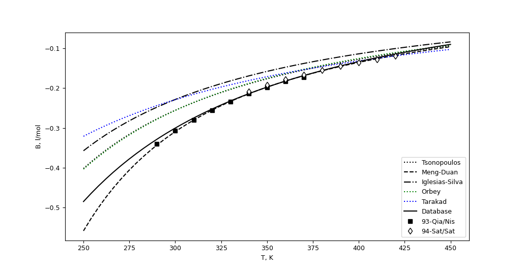
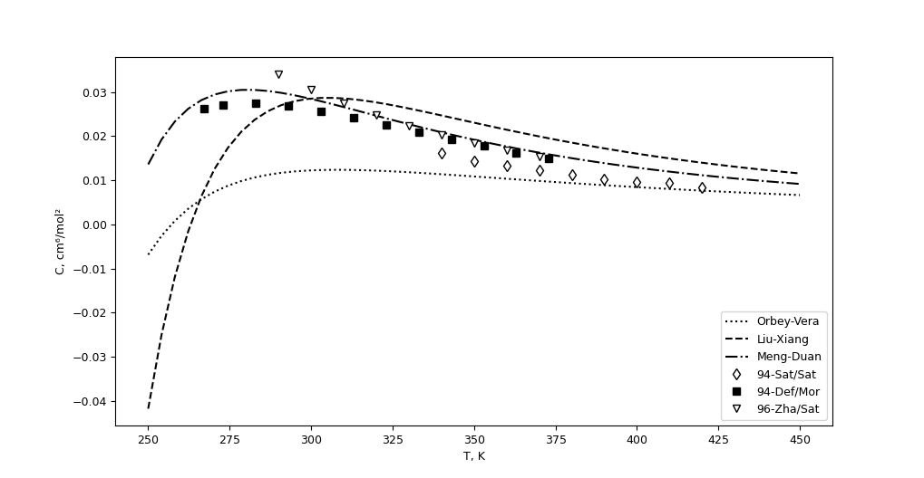
Example code of usage, plot the correlations for R32 and compare with some sources of experimental values

from matplotlib import pyplot
from numpy import linspace, r_

from lib.mEoS import R32
from lib.EoS import virial

D = R32.momentoDipolar.Debye
Vc = R32.M/R32.rhoc

# 2nd virial coefficient
B1 = []
B2 = []
B3 = []
B4 = []
B5 = []
B6 = []
coef = virial.B_Database[R32.id]

Ti = linspace(250, 450, 50)
for T in Ti:
    B1.append(virial.B_Tsonopoulos(T, R32.Tc, R32.Pc, R32.f_acent)[0])
    B2.append(virial.B_Meng(T, R32.Tc, R32.Pc, R32.f_acent, D)[0])
    B3.append(virial.B_IglesiasSilva(T, R32.Tc, R32.Pc, Vc, R32.f_acent, D)[0])
    B4.append(virial.B_Orbey(T, R32.Tc, R32.Pc, R32.f_acent, R32.id)[0])
    B5.append(virial.B_Tarakad(T, R32.Tc, R32.Pc, R32.id)[0])
    B6.append(virial._B_Database(T, coef)[0])
pyplot.plot(Ti, B1, label="Tsonopoulos", ls=":", c="k")
pyplot.plot(Ti, B2, label="Meng-Duan", ls="--", c="k")
pyplot.plot(Ti, B3, label="Iglesias-Silva", ls="-.", c="k")
pyplot.plot(Ti, B4, label="Orbey", ls=":", c="g")
pyplot.plot(Ti, B5, label="Tarakad", ls=":", c="b")
pyplot.plot(Ti, B6, label="Database", ls="-", c="k")

# Experimental date
# Qian, Z.Y., Nishimura, A., Sato, H., Watanabe, K.
# Compressibility Factors and Virial Coefficients of Difluoromethane
# (HFC-32) Determined by Burnett Method
# JSME Int. J. Ser. B. 36(4) (1993) 665-670
T = [290, 300, 310, 320, 330, 340, 350, 360, 370]
B = r_[-0.33975, -0.30666, -0.28011, -0.25594, -0.23379, -0.21422,
       -0.19777, -0.18327, -0.17231]
pyplot.plot(T, B, ls='', marker="s", mec="k", mfc="k", label="93-Qia/Nis")

# Sato, T., Sato, H., Watanabe, K.
# PVT Property Measurements for Difluromethane
# J. Chem. Eng. Data 39(4) (1994) 851-854
T = [340, 350, 360, 370, 380, 390, 400, 410, 420]
B = r_[-207.9, -191.4, -178.2, -166.2, -155.2, -144.7, -135.6, -128.1,
       -119.5]*1e-3
pyplot.plot(T, B, ls='', marker="d", mec="k", mfc="w", label="94-Sat/Sat")

pyplot.ylabel("B, l/mol")
pyplot.xlabel("T, K")
pyplot.legend()
pyplot.show()

from matplotlib import pyplot
from numpy import linspace, r_
from scipy.constants import R

from lib.EoS import virial
from lib.mEoS import R32

Zc = R32.Pc/R32.rhoc/R*R32.M/R32.Tc/1000
D = R32.momentoDipolar.Debye

# 3rd Virial coefficient
C1 = []
C2 = []
C3 = []
Ti = linspace(250, 450, 50)
for T in Ti:
    C1.append(virial.C_OrbeyVera(T, R32.Tc, R32.Pc, R32.f_acent)[0]*1e6)
    C2.append(virial.C_LiuXiang(T, R32.Tc, R32.Pc, R32.f_acent, Zc)[0]*1e6)
    B = virial.B_Meng(T, R32.Tc, R32.Pc, R32.f_acent, D)
    C3.append(virial.C_Meng(T, R32.Tc, R32.Pc, D, B)[0]*1e6)

pyplot.plot(Ti, C1, ls=":", c="k", label="Orbey-Vera")
pyplot.plot(Ti, C2, ls="--", c="k", label="Liu-Xiang")
pyplot.plot(Ti, C3, ls="-.", c="k", label="Meng-Duan")

# Sato, T., Sato, H., Watanabe, K.
# PVT Property Measurements for Difluromethane
# J. Chem. Eng. Data 39(4) (1994) 851-854
T = [340, 350, 360, 370, 380, 390, 400, 410, 420]
C = r_[0.01625, 0.01431, 0.01325, 0.01226, 0.01133, 0.01034, 0.009646, 0.009418, 0.00848]
pyplot.plot(T, C, ls='', marker="d", mec="k", mfc="w", label="94-Sat/Sat")

# Defibaugh, D.R., Morrison, G., Weber, L.A.
# Thermodynamic Properties of Difluoromethane
# J. Chem. Eng. Data 39(2) (1994) 333-340
T = [267, 273, 283, 293, 303, 313, 323, 333, 343, 353, 363, 373]
C = r_[0.0263, 0.027, 0.0274, 0.0268, 0.0256, 0.0242, 0.0226, 0.0209, 0.0193, 0.0178, 0.0162, 0.0149]
pyplot.plot(T, C, ls='', marker="s", mec="k", mfc="k", label="94-Def/Mor")

# Zhang, H., Sato, H., Watanabe, K.
# Gas Phase PVT Properties for the Difluoromethane + Pentafluoroethane
# (R32+R125) System
# J. Chem. Eng. Data 41(6) (1996) 1401-1408
T = [290, 300, 310, 320, 330, 340, 350, 360, 370]
C = r_[0.0341, 0.0305, 0.0275, 0.0248, 0.0224, 0.0203, 0.0185, 0.0168, 0.0153]
pyplot.plot(T, C, ls='', marker="v", mec="k", mfc="w", label="96-Zha/Sat")

pyplot.ylabel("C, cm⁶/mol²")
pyplot.xlabel("T, K")
pyplot.legend()
pyplot.show()

Other correlations don’t implemented¶

Romero-Lielmezs (1989)¶

Correlation for second virial coefficient using the Redlich-Kwong cubic EoS. The correlation need the compound dependent coefficient x.

\[\begin{split}\begin{array}[t]{l} B_r = \frac{BP_c}{RT_c} \\ B_r = \Omega_b - \Omega_a \frac{\alpha}{T_r} \\ \alpha(T_r, \omega, \mu_r^x) = \alpha^{(0)}(T_r) + \omega\alpha^{(1)}(T_r) + \mu_r^x\alpha^{(2)}(T_r) \\ \alpha^{(0)} = -1.4524905 + 14.360017/T_r - 45.000285/T_r^2 + 14.078304/T_r^6 + 1.7835426/T_r^7 \\ \alpha^{(1)}(T_r) = -4.3816022 + 15.205023/T_r - 20.874489/T_r^2 + 12.697209/T_r^3 - 2.5851848/T_r^4 \\ \alpha^{(2)}(T_r) = -0.008019636/T_r^7 + 0.01092317/T_r^8 - 0.003505639/T_r^9 \\ \end{array}\end{split}\]

Romero, A., Lielmezs, J. Correlation of Second Virial Coefficient for Polar Fluids. Thermochimica Acta 145 (1989) 257-264, http://dx.doi.org/10.1016/0040-6031(89)85145-7.

Besher-Lielmezs (1992)¶

Correlation for third virial coefficient using the Peng-Robinson cubic EoS. The correlation need the compound dependent coefficient x.

\[\begin{split}\begin{array}[t]{l} C_r = C \left(\frac{P_c}{RT_c}\right)^2 \\ C_r = \Omega_b^2 + 2\Omega_a \Omega_b F(T_r, \omega, \mu_r^x) \\ F(T_r, \omega, \mu_r^x) = F^{(0)}(T_r) + \omega F^{(1)}(T_r) + \mu_r^xF^{(2)}(T_r) \\ F^{(0)}(T_r) = -0.01175 - 0.80483/T_r + 7.29366/T_r^2 - 16.98304/T_r^3 + 16.86138/T_r^4 - 5.94613/T_r^5 \\ F^{(1)}(T_r) = 9.25492 - 65.50763/T_r + 162.02620/T_r^2 - 183.23773/T_r^3 + 96.85253/T_r^4 - 19.08807/T_r^5 \\ F^{(2)}(T_r) = -1.30215 + 6.56985/T_r - 13.08120/T_r^2 + 12.85166/T_r^3 - 6.24687/T_r^4 + 1.20561/T_r^5 \\ \end{array}\end{split}\]

Besher, E.M., Lielmezs, J. Correlation for the third virial coefficient for non-polar and polar compounds using a cubic equation of state. Thermochimica Acta 200 (1992) 1-13, http://dx.doi.org/10.1016/0040-6031(92)85101-z.

Chueh-Prausnitz (1967)¶

Correlation for third virial coefficient. The correlation need the compound dependent coefficient d, give in paper for few compound.

\[\frac{C}{V_c^2} = \left(0.232T_R^{-0.25} + 0.468T_R^{-5}\right) \left(1-e^{1-1.89T_R^2}\right) + d e^{-2.49+2.3T_R-2.7T_R^2}\]

Chueh, P.L., Prausnitz, J.M. Third Virial Coefficients of Nonpolar Gases and Their Mixtures. AIChE J. 13(5) (1967) 896-902, http://dx.doi.org/10.1002/aic.690130516.

de Santis-Grande (1979)¶

Correlation for third virial coefficient. The correlation need two aditional molecular parameters as dipole polarizability and bondi molecular volume. The paper give these parameters for several compounds but not very much.

\[\begin{split}\begin{array}[t]{l} \frac{C}{v_c^2} = C^0(T_R) + dC´(T_R) + d^2C"(T_R) \\ C^0 = \frac{0.1961}{T_R^{0.25}} + \frac{0.3972}{T_R^5} + \left(0.06684T_R^4 - \frac{0.5428}{T_R^6}\right) e^{-T_R^2} \\ C´ = \frac{64.5}{T_R^9} \left(1-2.085 e^{-T_R^2}\right) \\ C" = \frac{801.7}{T_R^7} \\ d = \frac{\omega \alpha N}{b} \end{array}\end{split}\]

de Santis, R., Grande, B. An Equation for Predicting Third Virial Coeffcients of Nonpolar Gases. AIChE J. 25(6) (1979) 931-938, http://dx.doi.org/10.1002/aic.690250603.

lib.EoS.virial._B_Database(T, args)[source]¶

Calculate second virial coefficient, its 1st and 2nd temperature derivarives from coefficient in database

Parameters:

Tfloat: Temperature, [K]
argslist: Array with polinomial coefficient

Returns:

Bfloat: Second virial coefficient [dm³/mol]
Btfloat: T(∂B/∂T) [dm³/molK]
Bttfloat: T²(∂²B/∂T²) [dm³/molK²]

lib.EoS.virial.B_Tsonopoulos(T, Tc, Pc, w, mu=None)[source]¶

Calculate the 2nd virial coefficient using the Tsonopoulos correlation

\[\frac{BP_c}{RT_c} = f^{(0)}+\omega f^{(1)}+f^{(2)}+f^{(3)}\]

\[f^{(0)} = 0.1445 - \frac{0.33}{T_r} - \frac{0.1385}{T_r^2} - \frac{0.0121}{T_r^3} - \frac{0.000607}{T_r^8}\]

\[f^{(1)} = 0.0637 - \frac{0.331}{T_r^2} - \frac{0.423}{T_r^3} - \frac{0.008}{T_r^8}\]

\[f^{(2)} = \frac{a}{T_r^6}\]

\[f^{(3)} = \frac{b}{T_r^8}\]

\[a = -2.14e-4\mu_r-4.308e-21*\mu_r^8\]

\[b = 0.00908+0.0006957*\mu_r\]

Parameters:

Tfloat: Temperature [K]
Tcfloat: Critical temperature [K]
Pcfloat: Critical pressure
wfloat: Acentric factor [-]
mufloat, optional: dipole moment [debye]

Returns:

Bfloat: Second virial coefficient [dm³/mol]
Btfloat: T(∂B/∂T) [dm³/molK]
Bttfloat: T²(∂²B/∂T²) [dm³/molK²]

Notes

With the B_database this correlation is only for completeness, the a, b correlations are general and possibly not applicable to the compounds not availables in the B_database

References

[3] Tsonopoulos, C.; An Empirical Correlation of Second Virial Coefficients. AIChE Journal 20(2) (1974) 263-272

Examples

Selected date from Table 2, pag 74 for neon

>>> from lib.mEoS import Ne
>>> D = Ne.momentoDipolar
>>> "%0.4f" % B_Tsonopoulos(262, Ne.Tc, Ne.Pc, Ne.f_acent, D)[0]
'0.0113'

lib.EoS.virial.B_IglesiasSilva(T, Tc, Pc, Vc, w, D)[source]¶

Calculate the 2nd virial coefficient using the Iglesias-Silva Hall: correlation

\[\frac{B}{b_o} = \left(\frac{T_B}{T}\right)^{0.2} \left[1-\left(\frac{T_B}{T}\right)^{0.8}\right] \left[\frac{B_c} {b_o\left(\left(T_B/T_C\right)^{0.2}-\left(T_B/T_C\right)\right)} \right]^{\left(T_c/T\right)^n}\]

\[\frac{B_C}{V_C} = -1.1747 - 0.3668\omega - 0.00061\mu_R\]

\[n = 1.4187 + 1.2058\omega\]

\[\frac{b_o}{V_C} = 0.1368 - 0.4791\omega + 13.81\left(T_B/T_C\right)^2 \exp\left(-1.95T_B/T_C\right)\]

\[\frac{T_B}{T_C} = 2.0525 + 0.6428\exp\left(-3.6167\omega\right)\]

Parameters:

Tfloat: Temperature [K]
Tcfloat: Critical temperature [K]
Pcfloat: Critical pressure, [Pa]
Vcfloat: Critical specific volume, [m³/mol]
wfloat: Acentric factor [-]
Dfloat: dipole moment [debye]

Returns:

Bfloat: Second virial coefficient [dm³/mol]
Btfloat: T(∂B/∂T) [dm³/molK]
Bttfloat: T²(∂²B/∂T²) [dm³/molK²]

References

[6] Iglesias-Silva, G.A., Hall K.R.; An Equation for Prediction and/or Correlation of Second Virial Coefficients. Ind. Eng. Chem. Res. 40(8) (2001) 1968-1974

Examples

Selected date from Table 2, pag 74 for neon

>>> from lib.mEoS import Ne
>>> Vc = Ne.M/Ne.rhoc
>>> D = Ne.momentoDipolar.Debye
>>> "%0.4f" % B_IglesiasSilva(262, Ne.Tc, Ne.Pc, Vc, Ne.f_acent, D)[0]
'0.0102'

lib.EoS.virial.B_Meng(T, Tc, Pc, w, D)[source]¶

Calculate the 2nd virial coefficient using the Meng-Duan-Li correlation

\[\frac{BP_c}{RT_c} = f^{(0)}+\omega f^{(1)} + f^{(2)}\]

\[f^{(0)} = 0.13356 - \frac{0.30252}{T_r} - \frac{0.15668}{T_r^2} - \frac{0.00724}{T_r^3} - \frac{0.00022}{T_r^8}\]

\[f^{(1)} = 0.17404 - \frac{0.15581}{T_r^2} + \frac{0.38183}{T_r^3} - \frac{0.44044}{T_r^3} - \frac{0.00541}{T_r^8}\]

\[f^{(2)} = \frac{a}{T_r^6}\]

\[a = -3.0309e-6\mu_r^2+9.503e-11\mu_r^4-1.2469e-15\mu_r^6\]

Parameters:

Tfloat: Temperature [K]
Tcfloat: Critical temperature [K]
Pcfloat: Critical pressure
wfloat: Acentric factor [-]
Dfloat: dipole moment [debye]

Returns:

Bfloat: Second virial coefficient [dm³/mol]
Btfloat: T(∂B/∂T) [dm³/molK]
Bttfloat: T²(∂²B/∂T²) [dm³/molK²]

References

[7] Meng, L., Duan, Y.Y. Li, L.; Correlations for Second and Third Virial Coefficients of Pure Fluids. Fluid Phase Equilibria 226 (2004) 109-120

Examples

Selected date from Table 2, pag 74 for neon

>>> from lib.mEoS import Ne
>>> D = Ne.momentoDipolar.Debye
>>> "%0.4f" % (B_Meng(262, Ne.Tc, Ne.Pc, Ne.f_acent, D)[0])
'0.0099'

lib.EoS.virial.B_Orbey(T, Tc, Pc, w, id=None)[source]¶

Calculate the 2nd virial coefficient using the Orbey correlation

\[\frac{BP_c}{RT_c} = f^{(0)} + \omega f^{(1)} + f^{(2)}\]

\[f^{(0)} = 0.1479 - \frac{0.3321}{T_r} - \frac{0.02907}{T_r^2} - \frac{0.06849}{T_r^3}\]

\[f^{(1)} = 0.2473 - \frac{0.6092}{T_r} + \frac{1.0749}{T_r^2} - \frac{0.7569}{T_r^3}\]

\[f^{(2)} = \frac{a}{T_r^7}\]

where a is compound dependend parameters

Parameters:

Tfloat: Temperature [K]
Tcfloat: Critical temperature [K]
Pcfloat: Critical pressure
wfloat: Acentric factor [-]
idinteger: Index of compound in database

Returns:

Bfloat: Second virial coefficient [dm³/mol]
Btfloat: T(∂B/∂T) [dm³/molK]
Bttfloat: T²(∂²B/∂T²) [dm³/molK²]

References

[8] Orbey, H.; A Four Parameter Pitzer-Curl Type Correlation of Second Virial Coefficients. Chemical Engineering Comm. 65(1) (1988) 1-19

Examples

Using same value of Tsonopoulos correlation as reference

>>> from lib.mEoS import Ne
>>> "%0.4f" % B_Orbey(262, Ne.Tc, Ne.Pc, Ne.f_acent)[0]
'0.0104'

lib.EoS.virial.B_Tarakad(T, Tc, Pc, id)[source]¶

Calculate the 2nd virial coefficient using the Tarakad-Danner: correlation

\[B^o = \frac{BP_c}{RT_c} = B_{simple}^o + B_{size-shape}^o + B_{polar}^o\]

\[B_{simple}^o = 0.1445 - \frac{0.33}{T_r} - \frac{0.1385}{T_r^2} - \frac{0.0121}{T_r^3} - \frac{0.000607}{T_r^8}\]

\[B_{size-shape}^o = \left(-0.00787 + \frac{0.0812}{T_R^2} - \frac{0.0646}{T_R^3}\right)R - \left(\frac{0.00347}{T_R^2} - \frac{0.000149}{T_R^7}\right)R^2\]

\[B_{polar}^o = -\frac{0.028}{T_r^7}\Psi\]

Parameters:

Tfloat: Temperature [K]
Tcfloat: Critical temperature [K]
Pcfloat: Critical pressure
idinteger: Index of compound in database

Returns:

Bfloat: Second virial coefficient [dm³/mol]
Btfloat: T(∂B/∂T) [dm³/molK]
Bttfloat: T²(∂²B/∂T²) [dm³/molK²]

References

[9] Tarakad, R.R., Danner, R.P.; An Improved Corresponding States Method for Polar Fluids: Correlation of Second Virial Coefficients. AIChE J. 23(5) (1977) 685-695

Examples

Using same value of Tsonopoulos correlation as reference

>>> from lib.mEoS import Ne
>>> "%0.4f" % B_Tarakad(262, Ne.Tc, Ne.Pc, Ne.id)[0]
'0.0117'

lib.EoS.virial.C_OrbeyVera(T, Tc, Pc, w)[source]¶

Calculate the third virial coefficient using the Orbey-Vera correlation

\[\frac{CP_c^2}{R^2T_c^2} = f^{(0)} + f^{(1)}\omega\]

\[f^{(0)} = 0.01407+\frac{0.02432}{T_r^{2.8}}-\frac{0.00313}{T_r^{10.5}}\]

\[f^{(1)} = -0.02676+\frac{0.0177}{T_r^{2.8}}+\frac{0.04}{T_r^3} -\frac{0.003}{T_r^6}-\frac{0.00228}{T_r^{10.5}}\]

Parameters:

Tfloat: Temperature [K]
Tcfloat: Critical temperature [K]
Pcfloat: Critical pressure
wfloat: Acentric factor [-]

Returns:

Cfloat: Third virial coefficient [dm⁶/mol²]
C1float: T(∂C/∂T) [dm⁶/mol²]
C2float: T²(∂²C/∂T²) [dm⁶/mol²]

References

[4] Orbey, H., Vera, J.H.; Correlation for the Third Virial Coefficient Using Tc, Pc and ω as Parameters. AIChE Journal 29(1) (1983) 107-113

Examples

Selected points from Table 2 of paper

>>> from lib.mEoS.Benzene import Benzene as Bz
>>> "%.1f" % (C_OrbeyVera(0.877*Bz.Tc, Bz.Tc, Bz.Pc, Bz.f_acent)[0]*1e9)
'41.7'
>>> "%.1f" % (C_OrbeyVera(1.019*Bz.Tc, Bz.Tc, Bz.Pc, Bz.f_acent)[0]*1e9)
'36.0'

lib.EoS.virial.C_LiuXiang(T, Tc, Pc, w, Zc)[source]¶

Calculate the third virial coefficient using the Liu-Xiang correlation

\[\frac{CP_c^2}{R^2T_c^2} = f^{(0)} + \omega f^{(1)} + \theta f^{(2)}\]

\[\theta = \left(Z_c-0.29\right)^2\]

\[f^{(0)} = a_{00} + \frac{a_{10}}{T_r^3} + \frac{a_20}{T_r^6} + \frac{a_{30}}{T_r^{11}}\]

\[f^{(1)} = a_{01} + \frac{a_{11}}{T_r^3} + \frac{a_21}{T_r^6} + \frac{a_{31}}{T_r^{11}}\]

\[f^{(2)} = a_{02} + \frac{a_{12}}{T_r^3} + \frac{a_22}{T_r^6} + \frac{a_{32}}{T_r^{11}}\]

Parameters:

Tfloat: Temperature [K]
Tcfloat: Critical temperature [K]
Pcfloat: Critical pressure
wfloat: Acentric factor [-]
Zcfloat: Critical compresibility factor [-]

Returns:

Cfloat: Third virial coefficient [dm⁶/mol²]
C1float: T(∂C/∂T) [dm⁶/mol²]
C2float: T²(∂²C/∂T²) [dm⁶/mol²]

References

[5] Liu, D.X., Xiang, H.W.; Corresponding-States Correlation and Prediction of Third Virial Coefficients for a Wide Range of Substances. Int. J. Thermophysics 24(6) (2003) 1667-1680

lib.EoS.virial.C_Meng(T, Tc, Pc, D, B)[source]¶

Calculate the 3rd virial coefficient using the Meng-Duan-Li correlation

\[\frac{CP_c^2}{R^2T_c^2} = 5.476e-3 + \left(\frac{BP_c}{RT_c}-0.0936 \right)^2 \left(f^{(0)} + \mu_r^4 f^{(1)}x10^{-10}\right)\]

\[f^{(0)} = 1094.051 - \frac{3334.145}{T_r^{0.1}} + \frac{3389.848}{T_r^{0.2}} - \frac{1149.58}{T_r^{0.3}}\]

\[f^{(1)} = 2.0243 - \frac{0.85902}{T_r}\]

Parameters:

Tfloat: Temperature [K]
Tcfloat: Critical temperature [K]
Pcfloat: Critical pressure
Dfloat: dipole moment [debye]
Blist: Second virial coefficient tuple with B, ∂B/∂T, ∂²B/∂T²

Returns:

Cfloat: Third virial coefficient [dm⁶/mol²]
C1float: T(∂C/∂T) [dm⁶/mol²]
C2float: T²(∂²C/∂T²) [dm⁶/mol²]

References

[7] Meng, L., Duan, Y.Y. Li, L.; Correlations for Second and Third Virial Coefficients of Pure Fluids. Fluid Phase Equilibria 226 (2004) 109-120

class lib.EoS.virial.Virial(*args, **kwargs)[source]¶

Bases: EoS

Class to model the virial equation of state

\[Z = \frac{PV}{RT} = 1 + \frac{B}{V} + \frac{C}{V^2} + \cdots\]

The implementation use the form truncated at third term using the virial coefficient from database or try to predicted from reference correlations. This equation is only appropiate for single-phase gas systems.

Methods

`B`(T)	Second virial coefficient calculation
`C`(T)	Third virial coefficient calculation

METHODS_B = ['Tsonopoulos (1974)', 'Iglesias-Silva (2001)', 'Meng (2004)']¶

METHODS_C = ['Orbey-Vera (1983)', 'Liu-Xiang (2003)', 'Meng (2004)']¶

__init__(*args, **kwargs)[source]¶

_Bi(T)[source]¶: Second virial coefficient muxture contributions

_Ci(T)[source]¶: Third virial coefficient mixture contributions

B(T)[source]¶: Second virial coefficient calculation

C(T)[source]¶: Third virial coefficient calculation

_physics(T, P, mezcla)[source]¶: Properties of Gases calculation. Explanation in [1] section 1.4

_fug(Z, xi)[source]¶: Calculate partial fugacities coefficieint of components, Eq 6-7.9

lib.EoS.virial module¶

Other correlations don’t implemented¶

Romero-Lielmezs (1989)¶

Besher-Lielmezs (1992)¶

Chueh-Prausnitz (1967)¶

de Santis-Grande (1979)¶

References¶

Table of Contents

Previous topic

Next topic

This Page